Power Query: Data Transformation of Dynamic Columns

When you manually select all columns and apply a transformation (for example, changing the data type) the generated code lists each column name individually – it looks something like this:

// Generated code from manual actions
=   Table.TransformColumnTypes ( 
        #"Previous Step",
        {
            {"First Column", type text}, 
            {"2nd Column", type text}, 
            {"Col 3", type text}, 
            {"COLUMN FOUR", type text}, 
            {"Number Five (is alive)", type text}, 
            {"666", type text}
        }
    )

I frequently import data from files with varying column names, and / or varying numbers of columns. This makes it impossible to effectively hard code data transformations by column name – if somebody renames any of those columns, then the step above will fail.

So, instead of the generated steps to change each column type, we can use the List.Transform function to apply a transformation to each Column:

//Change All Columns to text
=   Table.TransformColumnTypes ( 
        #"Previous Step", 
        List.Transform ( 
            Table.ColumnNames ( #"Previous Step" ), 
            each {_, type text}
        )
    )

This example is about as simple as it gets – you can of course apply a broad range of transformation functions in this way – for example, Text.Trim:

//Trim All Columns
=   Table.TransformColumns ( 
        #"Previous Step", 
        List.Transform ( 
            Table.ColumnNames ( #"Previous Step" ), 
            each {_, Text.Trim, type text}
        )
    )

Excel Book Recommendation

I am often asked to recommend an Excel book. This isn’t always easy, as different people need different things from a book, depending not only on their Excel ability and aspirations, but also their personality and learning preferences.

Excel 2010 BibleOne consistent recommendation I do give, though, is for John Walkenbach’s Excel Bibles:
Excel 2010 Bible – John Walkenbach – Amazon UK


If you only want to get ONE Excel book, this would be it. There’s a bible for each version of Excel, and they’re an excellent mix of how-to guides, background information and reference material.


Write Excel Data to Text File – Early Binding

Following on from my last post Using VBA to Write Excel Data to Text File – I’ve had this reply from Bernie Deitrick, Excel MVP, who has written a modified version of the code for when early binding is preferred:

Sub WriteTextFileEarlyBinding()
    Dim rng As Range
    Dim lRow As Long
    Dim strOutput As String
    Dim strNextLine As String
    Dim strFilename As String
    Dim strSeparator
    Dim adStream As ADODB.Stream

    'CHANGE THESE PARAMETERS
    strFilename = ThisWorkbook.Path & "\Output.txt"
    Set rng = ActiveSheet.UsedRange    'Selection
    strSeparator = vbTab   ' e.g. for comma seperated value, change this to strSeparator = ","

    For lRow = 1 To rng.Rows.Count
        strNextLine = Join$(Application.Transpose(Application.Transpose(rng.Rows(lRow).Value)), strSeparator)
        If strOutput = "" Then
            strOutput = strNextLine
        Else
            strOutput = strOutput & vbCrLf & strNextLine
        End If
    Next lRow

    Set adStream = New ADODB.Stream

    With adStream
        .Type = adTypeText  ' or use adTypeBinary
        .Charset = "us-ascii"    'See table below
        .Open
        .WriteText strOutput
        .SaveToFile strFilename, adSaveCreateOverWrite    ' 2; adSaveCreateNotExist = 1
    End With

End Sub

'Constant            Value
'CdoBIG5            "big5"
'CdoEUC_JP          "euc-jp"
'CdoEUC_KR          "euc-kr"
'CdoGB2312          "gb2312"
'CdoISO_2022_JP     "iso-2022-jp"
'CdoISO_2022_KR     "iso-2022-kr"
'CdoISO_8859_1      "iso-8859-1"
'CdoISO_8859_2      "iso-8859-2"
'CdoISO_8859_3      "iso-8859-3"
'CdoISO_8859_4      "iso-8859-4"
'CdoISO_8859_5      "iso-8859-5"
'CdoISO_8859_6      "iso-8859-6"
'CdoISO_8859_7      "iso-8859-7"
'CdoISO_8859_8      "iso-8859-8"
'CdoISO_8859_9      "iso-8859-9"
'cdoKOI8_R          "koi8-r"
'cdoShift_JIS       "shift-jis"
'CdoUS_ASCII        "us-ascii"
'CdoUTF_7           "utf-7"
'CdoUTF_8           "utf-8"
'The contents of Charset are case-insensitive. The default value is "us-ascii".

Code posted with his permission. Thanks, Bernie!

Using VBA to Write Excel Data to Text File

It’s a fairly common requirement to need a bit of VBA code to write Excel data to a text file.  There are several methods you can use to do this, but here’s an example which I like to use, as it offers good control over the range of data, the structure and format of the text output and – unusually – control over the text encoding / character set. It is really simple to specify UTF-8, UTF-16, ASCII, ISO8859, etc.

Sub WriteTextFile()

Dim rng As Range, lRow As Long
Dim stOutput As String, stNextLine As String, stSeparator As String
Dim stFilename As String, stEncoding As String
Dim fso As Object

'-------------------------------------------------------------------------------------
'CHANGE THESE PARAMETERS TO SUIT
Set rng = ActiveSheet.UsedRange 'this is the range which will be written to text file
stFilename = "C:\Temp\TextOutput.txt" 'this is the text file path / name
stSeparator = vbTab 'e.g. for comma seperated value, change this to ","
stEncoding = "UTF-8" 'e.g. "UTF-8", "ASCII"
'-------------------------------------------------------------------------------------

For lRow = 1 To rng.Rows.Count
    If rng.Columns.Count = 1 Then
        stNextLine = rng.Rows(lRow).Value
    Else
        stNextLine = Join$(Application.Transpose(Application.Transpose(rng.Rows(lRow).Value)), stSeparator)
    End If
    If stOutput = "" Then
        stOutput = stNextLine
    Else
        stOutput = stOutput & vbCrLf & stNextLine
    End If
Next lRow

Set fso = CreateObject("ADODB.Stream")
With fso
    .Type = 2
    .Charset = stEncoding
    .Open
    .WriteText stOutput
    .SaveToFile stFilename, 2
End With
Set fso = Nothing

End Sub

Change the parameters to suit your needs – you can use any code you like in this section, as long as the four variables rng, stFilename, stSeparator and stEncoding are assigned.


How to Unpivot Excel Data

All too often, data gets stored in crosstab format in Excel. Whilst crosstabs can be great for presenting data, they’re pretty poor for storing it, as it makes it tricky to manipulate the data. Therefore we often have a requirement to ‘unpivot’, or normalise the data. This is a quick tutorial of one method to unpivot Excel data.

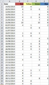
Here’s an example of what we’re working with. This is some meaningless, imaginary data, showing some values grouped in a crosstab by colour columns, and by date rows:

Unpivot Excel data - raw crosstab data

Whilst this seems like a reasonable way to store the information, it actually makes it pretty difficult to answer questions about this data – for example, what percentage of September values were Red?

What we really want is for each row to contain only one value, and for colour to be a column field. Then we can easily use a pivot table to interrogate this data.

We’re going to use a Multiple Consolidation Range pivot table to do the hard work for us.

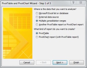
1. Start off by pressing keys ALT > D > P to open the Pivot Table Wizard dialog box:

Unpivot Excel data - Pivot Wizard Step 1

Choose the ‘Multiple consolidation ranges’ option, then click ‘Next’

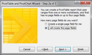
2a. In step 2a of the wizard, choose the ‘I will create the page fields’ option, and click ‘Next’

Unpivot Excel data - Pivot WIzard Step 2a


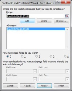
2b. Now we need to add our crosstab data range as a data source for this pivot table. Enter / select the appropriate range, then click ‘Add’. Then click ‘Next’.

Unpivot Excel data - Pivot Wizard Step 2b


3. Choose a location for the intermediate pivot table (it’s a good idea to use a new worksheet, as we can simply delete the entire worksheet when we’re finished). Then click ‘Finish’.

Unpivot Excel data - Pivot Wizard Step 3


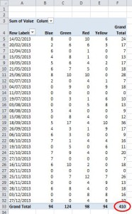
4. We now have an ‘intermediate’ pivot table, which looks very similar to our raw data, but has some grand totals. Now we want to drill into the source data for this pivot table, by double clicking on the overall Grand Total value – the cell intersection of the Grand Total column, and Grand Total row – circled red:

Unpivot Excel data - Intermediate pivot table


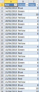
5. By double clicking to drill into the grand total data source, another worksheet is created, containing a table with our unpivotted data:

Unpivot Excel data - Unpivotted data

You can see that we now have colour as a column field, rather than four separate column headings – which allows us to use this data as a field in a pivot table report.

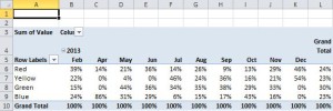
So, returning to our original example question – what percentage of September values were red? – it is now easy to put a quick pivot table together to answer this:

Unpivot Excel data - Pivot table report output

This is one method to unpivot Excel Data, which works well for simple crosstabs. It won’t deal with all cases – for example, where you already have multiple row fields in your data – but for simple cases like this example dataset, it’s a really quick and easy way of making your data a bit more accessible.

Download Excel file Download Example Workbook


Reset Application

If you’re anything like me, you often have several workbook projects open at one time, a mix from barely developed to pre-deployment beta.

And again, if you’re as forgetful as I am, you have run into a situation where you’ve entered debug part way through some faulty code, been distracted by something else and forgotten that the code which was running had disabled screenupdating, or events, or similar. Then switched blithely to another workbook, and been puzzled as to why your events aren’t firing, or why nothing is calculating as it should… Then spent ages pondering over perfectly good code, only to eventually remember that your last routine aborted and left events disabled. Or a cryptic progress message in your status bar. Or no error messages displaying ever again…

Well, maybe it’s only me! But, in case you recognise this, here’s a tip:

Sub ResetApplication()
    If Application.Workbooks.Count = 1 Then
        MsgBox "There are no open workbooks." & vbCr & vbCr & "Application cannot be reset.", vbExclamation + vbOKOnly, "XLSM | Invalid Procedure / Call"
        Exit Sub
    End If
    On Error GoTo ErrCatch
    With Application
        .DisplayAlerts = True
        .ScreenUpdating = True
        .EnableEvents = True
        .Calculation = xlCalculationAutomatic
        .StatusBar = False
        .DisplayFullScreen = False
    End With
    Err.Clear
Exit Sub
ErrCatch:
    MsgBox "An unknown arror occured while running code in Personal.xlsb." & vbCr & vbCr & _
        "If this problem persists, throw the PC out of the window.", vbCritical + vbOKOnly, "XLSM | Error"
End Sub

A bit of code like this saved to your Personal Workbook, with a nice little icon in the QAT – quick access toolbar – means that when light begins to dawn that you carelessly left the application somewhat undone, you can restore more normal settings with a simple click.