Happy Power Query Christmas

(Names, Behaviours) =>
let
    #"Make List" = Table.FromColumns({Names,Behaviours}, {"Name", "Behaviour"}),
    #"Check Once" = Table.SelectRows(#"Make List", each ([Behaviour] <> "Naughty")),
    #"Check Twice" = Table.SelectRows(#"Check Once", each ([Behaviour] = "Nice")),
    #"Santa Claus" = if Table.RowCount(#"Check Twice") > 0 then "is coming to town" else null
in
    #"Santa Claus"

Power Query: Data Transformation of Dynamic Columns

When you manually select all columns and apply a transformation (for example, changing the data type) the generated code lists each column name individually – it looks something like this:

// Generated code from manual actions
=   Table.TransformColumnTypes ( 
        #"Previous Step",
        {
            {"First Column", type text}, 
            {"2nd Column", type text}, 
            {"Col 3", type text}, 
            {"COLUMN FOUR", type text}, 
            {"Number Five (is alive)", type text}, 
            {"666", type text}
        }
    )

I frequently import data from files with varying column names, and / or varying numbers of columns. This makes it impossible to effectively hard code data transformations by column name – if somebody renames any of those columns, then the step above will fail.

So, instead of the generated steps to change each column type, we can use the List.Transform function to apply a transformation to each Column:

//Change All Columns to text
=   Table.TransformColumnTypes ( 
        #"Previous Step", 
        List.Transform ( 
            Table.ColumnNames ( #"Previous Step" ), 
            each {_, type text}
        )
    )

This example is about as simple as it gets – you can of course apply a broad range of transformation functions in this way – for example, Text.Trim:

//Trim All Columns
=   Table.TransformColumns ( 
        #"Previous Step", 
        List.Transform ( 
            Table.ColumnNames ( #"Previous Step" ), 
            each {_, Text.Trim, type text}
        )
    )

Power Query – How To Paste Code (video)

Power Query is great at solving data transformation and consolidation issues. But there are still loads of Excel users who have never used Power Query yet – and sometimes when they’re given some Power Query code to answer their question, they don’t know what to do with it.

Here’s a short video explaining how to use that Power Query code you’ve been given.

Power Query & Power Pivot

I realise I haven’t posted anything on here in quite a long time. That’s mainly because I’ve spent a long time learning all about Power Excel – and it’s a brave new world!

I used to spend most of my Excel time in the VBA editor. These days, I find I spend all my Excel time using Power Query, and Power Pivot (and I wish Microsoft hadn’t changed their names in Excel 2016!)

Have you learned how to use these power tools, yet? If not, I strongly suggest you take some time to look into them. They make it possible to work with data SO much more easily than in the past, and they’re so much faster to learn and use than VBA / formula solutions.

It’s simple to mash up data from a variety of sources, to reshape it fo fit your requirement, and to join up multiple sources in one view. Creating robust measures in Power Pivot makes it much easier and more reliable for report consumers to modify their views and visualisations, safe in the knowledge that the numbers will stay right, and changing layouts won’t break any of the calculations! They provide a much more transparent solution too, which is easier to share, and to understand.

I’m planning to make some time soon to write some beginner’s guides to Power Query and Power Pivot – in the meantime, this is a great link, explaining some Power Query basics

Filter table, then delete filtered rows

It’s a pretty common requirement to filter out some values in an Excel table, then delete those rows from the table. It should be straightforward to do this with a little VBA, but it seems to catch lots of people out! Here’s one simple method:

Sub DelFilter()
    With MySheet
        With .ListObjects("MyTable").DataBodyRange
            .AutoFilter
            .AutoFilter Field:=4, Criteria1:="MyCriteria"
            .EntireRow.Delete
            .AutoFilter
        End With
    End With
End Sub

You just need to change the sheet codename, the table name, the field index number, and the criteria value.

It would be simple to replace the user selected values with variables or parameters, so the code becomes more reusable:

Sub TestDelFilter()
    Call DelFilterParam(Sheet1, "MyTable", 4, "MyCriteria")
End Sub


Sub DelFilterParam( _
    ByVal wsSheet As Worksheet, _
    ByVal stTable As String, _
    ByVal iField As Integer, _
    ByVal vCriteria As Variant)
    
    With wsSheet
        With .ListObjects(stTable).DataBodyRange
            .AutoFilter
            .AutoFilter Field:=iField, Criteria1:=vCriteria
            .EntireRow.Delete
            .AutoFilter
        End With
    End With
End Sub

This is a simple example, applying a very simple filter. But it’s usually the method for deleting the filtered rows which catches people out, and this approach makes it easy.

YTZ Dice Game in Excel

Here’s a “Yahtzee” style dice game in Excel; quickly developed, just for a bit of fun. Usual scoring rules apply – roll 5 dice up to 3 times, and score in each of the categories.

Click on dice number to “hold” that die, click on the blank score space to save roll score, then roll again. The high score table will show the 6 highest overall scores.

YTZ Game for Excel – click to download

Excel Book Recommendation

I am often asked to recommend an Excel book. This isn’t always easy, as different people need different things from a book, depending not only on their Excel ability and aspirations, but also their personality and learning preferences.

Excel 2010 BibleOne consistent recommendation I do give, though, is for John Walkenbach’s Excel Bibles:
Excel 2010 Bible – John Walkenbach – Amazon UK


If you only want to get ONE Excel book, this would be it. There’s a bible for each version of Excel, and they’re an excellent mix of how-to guides, background information and reference material.


Index / Match Formula – Basics

INDEX and MATCH are two of the most powerful and flexible functions in Excel – but they are also two of the least understood. I often meet users who are confident with VLOOKUP and HLOOKUP formulae, but don’t seem to understand INDEX and MATCH. So I thought I’d provide a basic guide to using these functions.

INDEX

This simply returns a value from a list, based on its position in the list.

The INDEX function requires 2 arguments; The first is the list of values, or range containing the list of values. The second argument is the position in that list from which to return a value.

Example Data

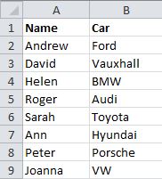
Example:  Who is the 4th name in this list? We can use INDEX to tell us:

=INDEX(A2:A9,4)

Which returns “Roger”.


MATCH

Now, the MATCH function does the exact opposite of INDEX: it returns the position in a list where a specific value occurs.

The MATCH function requires 3 arguments; The first is the value we want to find, the second is the list (or range containing the list) that we want to look in, and the third argument specifies whether we want an exact match, or the next lowest / highest.

Example DataExample: Which position is Helen in, in our example data:

=MATCH(“Helen”,A2:A9,0)

This formula returns the answer 3.

Note the third argument – 0 – which tells Excel we want an EXACT match.

INDEX / MATCH as a LOOKUP

These functions are each useful on their own. But when we combine them, they become even more powerful. Let’s look at the example data again, and ask the question:
Who drives the Hyundai?

Example DataNow, if the columns were reversed, you could simply use a VLOOKUP, to return the Name based on the Car value. So, you could restructure your data. Or you could add a helper column, to repeat the name in column C, and then use a VLOOKUP.

But it’s not always possible or practical to restructure a workbook, and it’s certainly not efficient to duplicate data. What we really want is a “left-looking” VLOOKUP – and this is where INDEX / MATCH can be used so effectively.

We can use MATCH to return the position in the list of Hyundai:
=MATCH(“Hyundai”,B2:B9,0)
This returns 6.

Now we can use the INDEX function to find the sixth name in the list:
=INDEX(A2:A9,6)
Which tells us it’s Ann.

Now we can simply combine the functions in one formula:
=INDEX(A2:A9,MATCH(“Hyundai”,B2:B9,0))
And with one little formula, we get the answer we wanted!

There are more advanced capabilities of both INDEX and MATCH functions, including 2 dimensional arrays, multiple areas, and returning closest values. But this post covers the basic use of the INDEX and MATCH functions in Excel.

Download Excel fileDownload Example File